MPI Primer

Fig. 1 illustrates a simplified version of how MPI sees a program. The view is process-centric. When the program starts, MPI defines a set MPI_COMM_WORLD which includes all of program’s processes. Within our example MPI_COMM_WORLD has three processes. MPI assigns these processes an integer value (ranging from 0 to “the number of processes minus 1”) called the process’s rank. More complicated MPI setups can have further partition MPI_COMM_WORLD into subsets, but the overall point remains: MPI’s view of a program is a series of processes somehow grouped together.

Fig. 1 Illustration of MPI’s runtime abstraction model.

In a typical MPI-based program parallelism is expressed by somehow mapping tasks and data to ranks. For example say we have three arbitrary functions foo, bar, and baz` and a chunk of data we want to run ``foo, bar, and baz on. Fig. 2 shows the three ways we can do this in parallel.

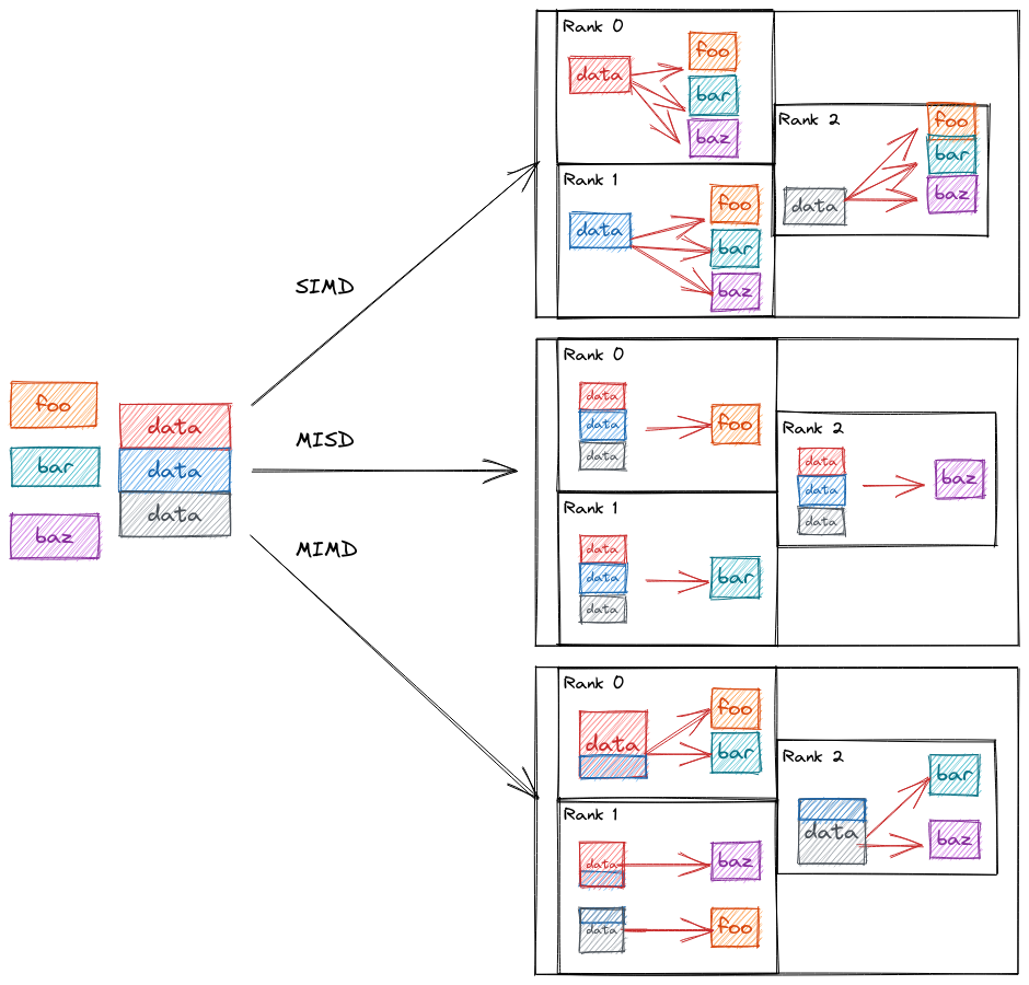
Fig. 2 Possible ways of mapping data and tasks to MPI ranks.

In the SIMD approach depicted at the top of Fig. 2 we distribute the data over the MPI ranks and have each rank pass its local chunk of data to the three functions. In MISD, which is shown in the middle of Fig. 2 we instead distribute the functions over the ranks. Finally, in the MIMD model shown at the bottom of Fig. 2 we distribute both the data and the functions.

Unfortunately on today’s machines it takes more than distributing tasks and/or data to otherwise opaque ranks to achieve high-performance. This is because the performance also depends on the hardware available to each rank and how well utilized that hardware is.