Designing the OpGraph
What is the OpGraph Component?
Program control flow is usually thought of in terms of graphs (specifically directed acyclic graph (DAG)s). Each node of the DAG is a task and edges indicate data dependencies/flow. Once the user has told TensorWrapper what they want to do, TensorWrapper converts that request into a DAG. The DAG is then passed to the backend which is then charged with traversing the DAG and executing the tasks it represents. Since the DAG generated by TensorWrapper will be comprised of tensor algebra operations, we term this DAG the “OpGraph”.
Why do we need an OpGraph?
Performing tensor algebra in a performant manner requires careful planning of the order tasks are done in, how they are done, and where they are done. In computer science we usually tackle this problem with DAGs. The OpGraph component is needed so that we can have a DAG representation of the user’s request. Thinking of the user’s inputs as a domain specific language (DSL) the OpGraph component is then the abstract syntax tree (AST) resulting from parsing the DSL (strictly speaking a concrete syntax tree (CST) actually results from parsing the DSL, which is then mapped to an AST, but that intermediate step is immaterial here). The association of the OpGraph component with an AST suggests another use: an intermediate representation of the calculation.
Expression Layer vs. OpGraph
Perhaps what is less clear is why do we need the expression layer AND the OpGraph component? This question is brought on by the fact that there is a fair amount of redundancy in the classes. Ultimately, the answer is a separation of concerns. The expression layer is purely meant to capture what the user wants to do. The OpGraph component is supposed to represent what TensorWrapper wants the backend to do. Generally speaking what the user wants to do will be expressed in terms of much coarser operations than what TensorWrapper wants the backend to do.
On a related note, another key difference between the Expression layer and the OpGraph component is the the Expression layer is designed so that it is easy for the user to express their intent, whereas the OpGraph is designed to be easy for a backend to traverse. Thus the Expression layer is equation-based whereas the OpGraph component is graph-based.
OpGraph Considerations
- data flow
The graph needs to be capable of distinguishing between inputs and outputs. There conceivably could be cycles if loops are involved.
- tensors appear multiple times
It is not uncommon for the same tensor to appear multiple times in a graph. For example many matrix decompositions are expressed in terms of a tensor and its transpose or a common intermediate may be used in several equations. The point is, we can not assume that all tensors in the graph are unique.
- multiple sources
The graph may have multiple inputs. The most obvious examples of this are binary operations, like addition, which map two input tensors to a single output tensor.
- Multiple sinks
The graph may have multiple results. A somewhat common example of this is an eigen solver which takes an input matrix, diagonalizes it, and returns the eigenvectors and the eigenvalues.
- data references
The
OpGraphmust either have handles to the actual data, or somehow be associated with the actual data in order for backends to translate the AST into results. But plainly, if we want the backend to add two tensors, we better give the backend the two tensors.
- expression compatibility
The
OpGraphobject will ultimately be filled in by the objects in the expression component. Thus the interface of theOpGraphclass needs to be designed so that it is compatible with theExpressioncomponent’s implementation (see Designing the Expression Component).As a corollary, this means that each
Expressionobject must be representable as part of the resultingOpGraph.
- extensible
While we will propose an initial set of basic operations, this set is not unique, nor will all backends agree that the operations are actually “basic”. An excellent example is tensor contraction, which most backends will actually further decompose into permutations and a gemm (the BLAS routine for general matrix multiplication). If at a later time we decide that we would like the
OpGraphto be able to express tensor contraction as permutations and a gemm, instead of a single operation, we will need to be able to add the ability to denote a gemm in theOpGraph.
- backend specific basic operations
Somewhat related to extensible not every backend will expose interfaces for every basic operation TensorWrapper knows about. We will need a mechanism of somehow knowing which basic operations a backend supports and a mechanism for rewriting an
OpGraphin terms of different operations.
Out of Scope
- Identifying unique/repeat tensors
The OpGraph component works with what it is given. If the OpGraph component is told that there are two tensors in the graph, the OpGraph component is going to assume there are two different tensors in the graph, and not a single tensor used twice. Identifying common intermediates should happen before forming the
OpGraph(or should be done as a transformation of theOpGraph).- Optimizing the OpGraph
Along the lines of identifying unique/repeat tensors, the OpGraph layer will not be responsible for optimizing the computations an
OpGraphobject represents. Optimizing the computations can be done by a layer which takes anOpGraphobject, analyzes it, and creates a new optimizedOpGraphobject.
Tensor Networks
The idea that tensor algebra can be expressed as a graph is not something new that we just stumbled on to. Mathematicians have known this for years. The graphical representation of tensor algebra is usually termed a “tensor network”. Here’s the basics (see References for background/where I took this from):
Nodes of a graph are tensors, edges are contractions.
The shape of the node can be used to convey properties of the tensor.
There seems to be several conventions in the wild.
Squares or circles are usually the default symbol and are drawn with the same area (vide infra).
Use of the default symbol indicates that no additional properties for the tensor are known/specified.
Tensors which result from combining other tensors are denoted with rectangles or ovals whose area reflects the total number of “default” tensors which were consumed.
Edges denote tensor modes.
The number of edges connected to a node equals the rank of that tensor.
Reshaping a tensor (typically flattening it) is done by combing edges into a single edge.
The thickness of the resulting edge is proportional to the number of modes comprising it. For example, reshaping a matrix into a vector would result in an edge which is twice as thick as the edges which were combined.
Edges can be labeled with dummy indices to make referring to a particular edge easier.
Contraction over multiple indices is denoted with parallel edges.
The trace of a tensor (or product of tensors) is denoted with a loop.
Additional operations, such as tensor products, addition, element-wise addition, etc. are usually specified with rectangles/ovals labeled with the operation.
The area rules specified above apply to the resulting node.
Tensor decompositions are usually represented by left and right pointing triangles (the left pointing triangle being the adjoint of the right pointing triangle). If the decomposition also results in “values”, e.g., eigenvalues or the singular values from a singular value decomposition, those values are represented by a square/circle between the triangles.
Why not use tensor networks for the OpGraph?
Tensor networks really seem to be geared at expressing contractions involving a number of tensors. While this is a very important use case for the OpGraph component, consideration expression compatibility requires that our graph also be capable of expressing other operations too. While tensor networks have a mechanism for this (recursive or hierarchical nodes, i.e., nodes which actually represent entire tensor networks themselves) this representation makes it hard to address consideration tensors appear multiple times. In particular, if the same tensor is involved in a contraction and say an addition, then it is difficult to express that it is indeed the same tensor (which in graph notation is naturally done by having it be literally the same node).
Another large problem with directly using a tensor network is tracking permutations. Tensor networks treat modes of a tensor as if only the number of modes (and the number of those modes which are contracted) matters. In practice, having to permute modes can have huge performance consequences and it must be considered (this is part of consideration expression compatibility). In theory this could be worked into the tensor network by enforcing an order to the edges (e.g., by requiring the edge for mode 0 to be the left most edge, the edge for mode 1 to be the second left most edge, etc.). Then permutations would manifest as edge crossings.
Ultimately, tensor networks were not designed to be task graphs, which is really what the OpGraph component is after. Tensor networks are useful for expressing the part of the task graph which maps to a specific tensor contraction, but beyond that they are cumbersome to manipulate when multiple terms are equations are involved. For this reason we have opted to generalize tensor networks.
OpGraph Notation
The graph represented by an OpGraph object can be considered a
generalization of a tensor network, with extensions to accommodate the extended
set of use cases the OpGraph component must deal with. The need for being able
to visualize an OpGraph object graphically is useful for design, and is
expected to also be useful for code analysis/optimization. To that end we
propose the following notation:
Nodes of the graph depict either tensors or operators.
Tensors are denoted with square nodes.
Operations with circles.
Nodes will be labeled with the name of the tensor or the operation.
Unlike traditional tensor networks, most operations are treated the same. The key exception is permutations which are carried on the edges instead of the nodes.
Edges denote modes.
Parallel edges are avoided by fusing indices, i.e., each edge is labeled with all indices participating in that operation.
The number of fused modes is tracked by annotating the modes.
The annotations are used to express permutations (and for the multiplication operation convey generalized Einstein summation convention).
Edges are directed.
The direction indicates data flow. Sources are input tensors. Sinks are outputs.
The rank of a tensor can be determined from the number of unique indices associated with it.
OpGraph Structure
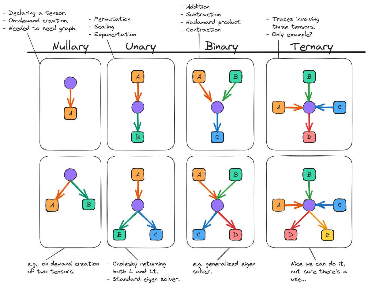
Fig. 15 Overview of how operations of different arity look using OpGraph graphical notation. For simplicity, mode annotations and operation labels are not specified.
Overview of how operations of different term_arity look using OpGraph
graphical notation. For simplicity, mode annotations and operation labels are
not specified. illustrates how an OpGraph representation looks for
operations of various arity. Graphs are grouped into a matrix such
that for row \(m\) (\(m\) is 1-based) the \(n\)-th column (\(n\) is 0-based) denotes an
operation returning \(m\) tensors given \(n\) tensors (\(m\) and \(n\) have different
bases because operations returning no tensors are not interesting).
The simplest, non-null, OpGraph stems from simply declaring a tensor. The
resulting “nullary” graph for a tensor \(\mathbf{A}\), is shown in Overview of how operations of different term_arity look using OpGraph
graphical notation. For simplicity, mode annotations and operation labels are
not specified.. From
the perspective of the OpGraph component, the actual declaration of a tensor
requires performing some opaque operation (such operations are denoted by purple
circles in Overview of how operations of different term_arity look using OpGraph
graphical notation. For simplicity, mode annotations and operation labels are
not specified.). For declaring a tensor this operation simply
returns the tensor (and does not require any input to do so, hence it is a
nullary operation). From the perspective of OpGraph, the nullary operations
which create the source tensors must always be present and they are not usually
interesting (effectively being lambdas like [](){return A;}). Thus by
convention, and in an effort to simplify the representation of OpGraph
objects, the nullary operations giving rise to the source tensors will usually
be implicit. The exception being when those nullary operations are interesting
(usually because they are on-demand generator functions). For the remaining
columns in Overview of how operations of different term_arity look using OpGraph
graphical notation. For simplicity, mode annotations and operation labels are
not specified. this convention applies. As shown in row 2 of
Overview of how operations of different term_arity look using OpGraph
graphical notation. For simplicity, mode annotations and operation labels are
not specified.
The next simplest OpGraph requires mapping an input tensor to an output
tensor via some intermediate operation. Such operations are “unary” and examples
include permuting the modes of a tensor, scaling a tensor, and raising a tensor
to a power. It is also possible that a unary operation returns multiple tensors,
e.g., a standard eigen solver which returns the eigenvectors and the
eigenvalues. At this point, the basic structure of an operation should be clear,
nonetheless Overview of how operations of different term_arity look using OpGraph
graphical notation. For simplicity, mode annotations and operation labels are
not specified. shows examples of some other arities.
Basic Operations
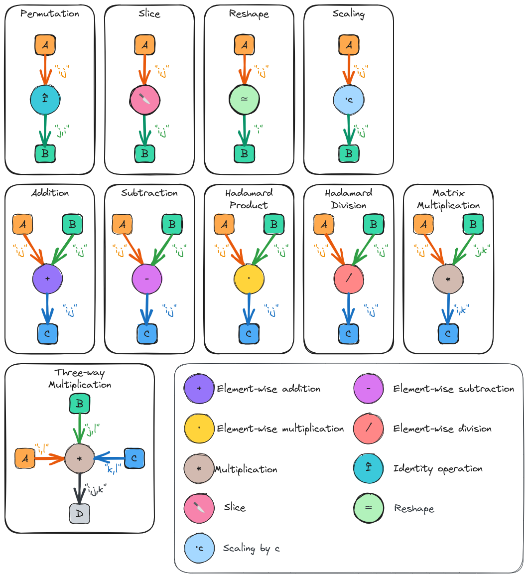
Fig. 16 Pictorial representations of the fundamental operations of the OpGraph component.
Pictorial representations of the fundamental operations of the OpGraph
component. shows some of the basic operations which will be
comprise actual OpGraph instances. For simplicity we have focused on matrix
operations (most input/output edges have two annotations), but much of what is
in Pictorial representations of the fundamental operations of the OpGraph
component. generalizes to other rank tensors in a
straightforward manner. Ignoring nullary operations, all operation nodes have
one or more inputs and one or more outputs. The goal is to establish a small set
of “fundamental” operations and to write all other operations in terms of these
operations. For example, we do not define a chip operation, but a chip operation
can be defined by a slice followed by a reshape.
As shown in Pictorial representations of the fundamental operations of the OpGraph component., tensors acting as inputs to an operation have their annotations associated with the edge connecting them to the operation. Tensors resulting from an operation have their annotations associated with the edge connecting the the operation to the tensor. In turn permutations are signified by reordering the output indices relative to the input indices.
The most questionable choice we have made is the “multiplication” operator. The multiplication operator actually stands in for a number of operations including trace, contraction, tensor product, and element-wise multiplication (though we have also defined an element-wise multiplication operator for consistency with the other element-wise operations). Our motivation here is that many of the backend tensor libraries have already invested in infrastructure for handling generalized Einstein summation convention (and/or tensor networks) and in the first pass we intend to dispatch to the backend’s implementations.
More Complicated OpGraphs
Ultimately, the state of an OpGraph is obtained by combining basic
operations from the previous subsection into larger graphs. From the
Designing the Expression Component section the first our more complicated
code examples was:
{
   auto aijk = a("i,j,k");
   c("i,j,k")  = aijk * b("i,j,k");
   d("i,j,k")  = aijk / b("i,j,k");
}
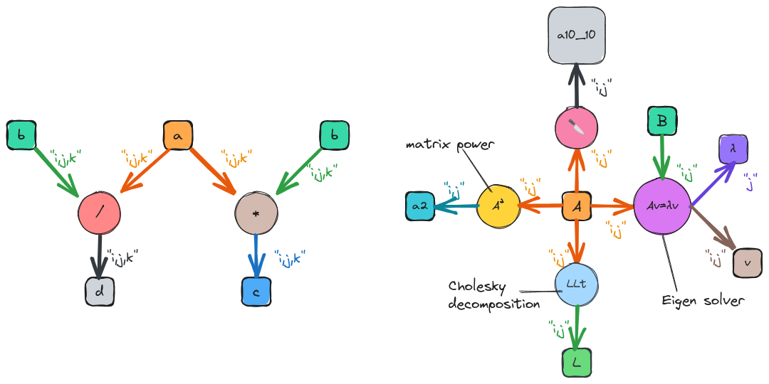
Fig. 17 Graphs resulting from the “complicated” code snippets.
The graph resulting from this code is shown on the left of
Graphs resulting from the “complicated” code snippets.. The graph expresses that after creation a is
used in two equations, which in turn result in two outputs. As was discussed
in Designing the Expression Component TensorWrapper will not be able to
identify common intermediates at first, so it treats b as two separate
tensors. The next most complicated code example we showed in
Designing the Expression Component was:
 T L, Lt, v, λ, a10_10, a2;
 {
     auto Aij = A("i,j");

    // disclaimer, I'm not 100% sure the cholesky/eigen_solve APIs will work
    // as shown, but it should be possible to get something close.

    // A = LLt
    L("i,j") = cholesky(Aij);

    // Av = λBv (no argument needed if B is 1)
    std::make_pair(v("i,j"), λ("j")]  = eigen_solve(Aij, B("i,j"));

    // Get the  slice of A starting a 0,0 and extending to 10,10 exclusive.
    a10_10("i,j") = slice(Aij, {0, 0}, {10, 10});

    // Raise A to the power 2
    a2("i,j") = pow(Aij, 2);
}
The graph resulting from this code snippet is shown on the right of
Graphs resulting from the “complicated” code snippets.. Here the intermediate A is used in four
different expressions including some expressions with multiple return values.
OpGraph Design
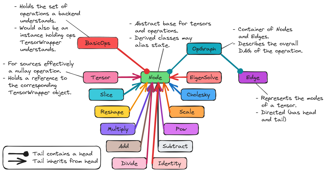
Fig. 18 The classes comprising
So far we have focused exclusively on the graph representation of the OpGraph and not the programmatic design. The classes comprising shows the classes comprising the OpGraph component of TensorWrapper. The classes are summarized in more detail in the following subsections
OpGraph
This is a container-like class which stores the actual DAG. The elements of the
OpGraph class are Edge and Node objects. The OpGraph object
additionally knows the connectivity of the graph and properties of the graph
(e.g., the number of sinks or sources).
Edge / Node
The fundamental elements of the OpGraph class are Edge and Node
objects. Edge objects represent tensor modes and the directionality of the
edge indicates whether a tensor is an input or an output. Node objects
represent either a tensor or an operation with tensors only being connected to
operations and operations only being connected to tensors (i.e., every
OpGraph is a bipartite graph).
BasicOps
Pursuant to consideration backend specific basic operations the OpGraph
component needs a way to be able to know what basic operations a backend can
handle. To this end we introduce the BasicOps class. The BasicOps class
is envisioned as being more or less a strong type over a std::set<Node>.
For each backend, TensorWrapper would maintain a BasicOps filled with the
operations that backend can parse. Before calling the backend with a specific
OpGraph TensorWrapper will ensue that the OpGraph is comprised entirely
of operations the backend understands. If it is not, TensorWrapper will either
rewrite the OpGraph in terms of operations the backend can understand or
error out.
Operations
The remaining classes in The classes comprising represent the basic
operations TensorWrapper knows about. Many of these classes are simply strong
types, although some, like Scale, will also contain state. By having the
various operations each have their own class we can address
data references. New operations can be added, thus satisfying the
extensible consideration, by
deriving new classes. The operations will only affect backends whose
corresponding BasicOps object is updated (thus preserving backwards
compatibility).
In satisfying expression compatibility we note that many classes in the Expression component have an analogous class in the OpGraph component. For those that don’t we explicitly note the mapping from the Expression component to the OpGraph component in the following list:
Indexedessentially maps to aTensornode plus anEdgeobject.ChipisSlicefollowed by a reshape.Permutationis determined by comparing the input and outputEdgeobjects.EigenVectorsandEigenValuesbecomeEigenSolveAssignTomaps to an edge stemming from a operationNode.
OpGraph API
Before discussing the API of the OpGraph component we want to remind the reader
that OpGraph objects will in general be generated by the expression layer. Hence
we fully expect users to interact with TensorWrapper through the expression
layer and will rely on the expression layer to generate OpGraph objects. In
turn, while the following code snippets are verbose we feel that is okay because
users will not be writing them.
The API of the OpGraph component is modeled after the Boost Graph Library
(see here). This
is to lower the barrier to entry in case the user is already familiar with that
library and so that an actual graph library (like Boost Graph Library) can be
wrapped by OpGraph if needed for performance.
The OpGraph class serves the role of an overall container for the graph. A
similar role to say boost::adjacency_matrix or boost::adjacency_list
classes.
using namespace opgraph; // OpGraph component lives in opgraph namespace

// Will be graph for A + B = C
OpGraph g;     // Default graph, no nodes

// Will be graph for pow(A, 2) = C
OpGraph g3(3); // Graph which will pre-allocate room for 3 nodes.

TensorWrapper A, B, C; // Assume these are set up already

// Creates three nodes which respectively represent tensor A, B, and C
g.add_node(Tensor{A}); // Will be node 0,
g.add_node(Tensor{B}); // node 1,
g.add_node(Add{});     // node 2,
g.add_node(Tensor{C}); // and node 3

g3.add_node(Tensor{A});
g3.add_node(Pow{2});  // Operation which squares a matrix
g3.add_node(Tensor(C));

g.add_edge(0, 2, "i,j"); // Adds an edge from node 0 to node 2 labeled "i,j"
g.add_edge(1, 2, "i,j"); // Similar, but edge goes from 1 to 2
g.add_edge(2, 3, "i,j"); // Similar, but edge goes from 2 to 3

g3.add_edge(0, 1, "i,j");
g3.add_edge(1, 2, "i,j");
Since Nodes can in general have the same value we can’t use the value of a node
as a “key” and we must refer to nodes by offset. For example, while an API like
g.add_edge(Tensor{A}, Add{}, "i,j"); would be user-friendly, if there were
say two add operations we wouldn’t know which Add instance to connect to
Tensor{A}. While it’s tempting to say that all Add instances are the
same, and thus we should just be connecting all addition operations to the same
node, doing so sacrifices the data dependency order (assume we only have a
single Add node, then if we add the output from an Add operation to
another tensor the resulting graph has a loop).
After we have created an OpGraph we can inspect it:
// Assume it's the same g from above

// Returns a pair of iterators over the nodes in the graph
auto [node_begin, node_end] = g.nodes();

// Returns a pair of iterators over the edges in the graph
auto [edge_being, edge_end] = g.edges();

// Number of nodes/edges
auto nnodes = g.num_nodes();
auto nedges = g.num_edges();

// The degree of a node is the total number of edges connected to it
assert(g.degree(0) == 1);
assert(g.degree(1) == 1);
assert(g.degree(2) == 3);
assert(g.degree(3) == 1);

//The in degree of a node is the number of nodes which feed into it
assert(g.in_degree(0) == 0);
assert(g.in_degree(1) == 0);
assert(g.in_degree(2) == 2);
assert(g.in_degree(3) == 1);

// The out degree is the number of nodes a node feeds in to
assert(g.out_degree(0) == 1);
assert(g.out_degree(1) == 1);
assert(g.out_degree(2) == 1);
assert(g.out_degree(3) == 0);

// Returns a pair of iterators over the edges connected to the specified
// node. Here node 0
auto [edges0_begin, edges0_end] = g.edges(0);
assert((*edges0_begin) == Edge(0, 1, "i,j")); // One edge going from 0 to 1

// Only the edges going in to node 0
auto [in_edges0_begin, in_edges0_end] = g.in_edges(0);
assert(in_edges0_begin == in_edges0_end); // There are none

// Only the edges going out of node 0
auto [out_edges0_begin, out_edges0_end] = g.out_edges(0);
assert((*out_edges0_begin) == Edge(0, 1, "i,j"));

// Returns a pair of iterators over the nodes connected to the specified
// node, here node 0
auto [nodes0_begin, nodes0_end] = g.adjacent_nodes(0);
assert((*nodes0_begin) == 2);

// OpGraph is a DAG so a pair of numbers maps to exactly one edge, *i.e.* :
assert(g.source(0, 2) == 0);
assert(g.source(2, 0) == 0);
assert(g.sink(0, 2) == 2);
assert(g.sink(2, 0) == 2);
While not shown, we anticipate that a series of free functions will be needed
for computing properties of OpGraph objects or running say depth-first
searches on them. We anticipate the such functions will wrap existing algorithms
supplied by the backend of the OpGraph component.
Summary
The design of the OpGraph component satisfies the above considerations by:
- data flow
Edges are directed and indicate whether the tensor connected to the edge is going into the operation or coming from it.
- tensors appear multiple times
The same
Tensorobject can be reused when an intermediate appears multiple times. Alternatively, differentTensorobjects can be created which point to the same intermediate.- multiple sources
Operations may have inputs which come from different tensors.
- Multiple sinks
Operations may point to (i.e. return) more than tensor.
- data references
The nodes of the graph are ultimately classes. Each operation is its own class and thus can store additional state if need be.
- expression compatibility
The initial design of the OpGraph component includes operations for most of the classes defined in the Expression component. For the remaining Expression component objects simple straightforward mappings to two or more OpGraph components exist.
- extensible
Additional operations can be added by deriving from the
Nodeclass.- backend specific basic operations
Each backend will be associated with a
BasicOpsobject which details the basic operations the backend can parse. Maintainers of TensorWrapper will be responsible for maintaining theBasicOpsobject.
References
For the tensor network background we primarily relied on sources found in the README of Google’s TensorNetwork project, specifically:
https://iopscience.iop.org/article/10.1088/1751-8121/aa6dc3/pdf
https://arxiv.org/pdf/1306.2164.pdf